Analysis Notebook
Contents
2.9. Analysis Notebook#
A copy of this notebook is run to analyse the molecular dynamics simulations.
2.9.1. Compound details#
This notebook refers to compound 33.
# show a 2d image of the molecule, and a 3d structure via py3dmol!
# also put sequence here.
According to the literature reference, there is only one distinct structure in solution.
2.9.2. Simulation details#
# Stereo check 1-frame trajectory to tmp-pdb file
t_stereo_check = topo.restrict_atoms(topo.topology.select('protein'))
tf = tempfile.NamedTemporaryFile(delete=False)
# tf.name
t_stereo_check.save_pdb(tf.name)
# Get reference mol
mol_ref = Chem.MolFromMol2File(snakemake.input.ref_mol, removeHs=False,)

# Get 1st frame pdb from tempfile
post_eq_mol = Chem.MolFromPDBFile(tf.name, removeHs=False, sanitize=False,)

# could compare smiles to automate the stereo-check. Problem: mol2 reference file has wrong bond orders
# (amber does not write those correctly). The ref-pdb file cannot be read b/c geometry is not optimized.
# This leads to funky valences in rdkit. The post-eq pdb file reads fine but then charges etc. dont match
# with the reference (b/c of wrong bond orders). But can manually check that all stereocentres are correct (below)
Chem.CanonSmiles(Chem.MolToSmiles(post_eq_mol)) == Chem.CanonSmiles(Chem.MolToSmiles(mol_ref))
False
post_eq_mol.RemoveAllConformers()
post_eq_mol
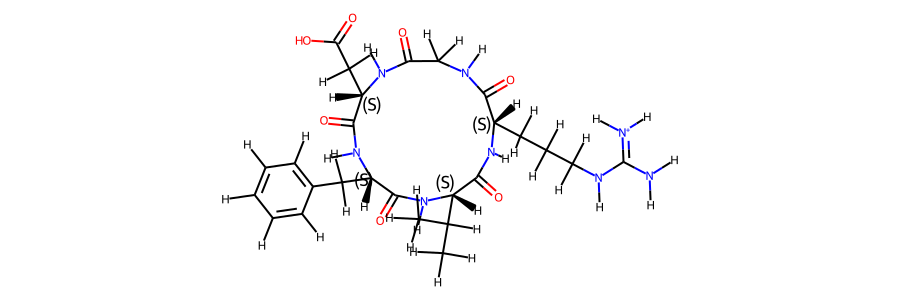
mol_ref.RemoveAllConformers()
mol_ref

The simulation type is GaMD, 2000 ns. The simulation was performed in H2O.
There are a total of 500000 frames available to analyse.
#determine stride to get 10k frames:
stride_short = int(t.n_frames / 10000)
if stride_short == 0:
    stride_short = 1

# save short trajectory to file
t[::stride_short].save_netcdf(snakemake.output.short_traj)

# this determines a cutoff for when we consider cis/trans conformers separately.
# only relevant if 2 sets of NOE values present.
# t.n_frames / 1000 -> 0.1% of frames need to be cis/trans to consider both forms.
CIS_TRANS_CUTOFF = int(t.n_frames / 1000)
However, for some of the analysis steps below, only 1% of these frames has been used to ensure better rendering in the browser.
2.9.3. Convergence of the simulation#
2.9.3.1. RMSD#
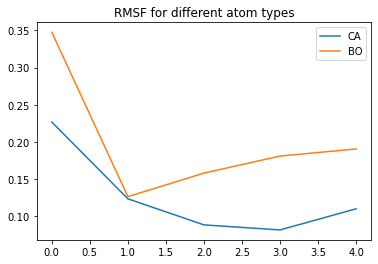
To check for convergence of the simulation, we can look at the root mean squared deviation of the atomic positions over the course of the simulation.
# RMSF might be interesting as well!
rmsf_ca = md.rmsf(t,t,0, ca)
rmsf_bo = md.rmsf(t,t,0, bo)

plt.plot(rmsf_ca, label='CA')
plt.plot(rmsf_bo, label='BO')
plt.legend()
plt.title('RMSF for different atom types')
plt.show()
2.9.3.2. Dihedral angles#
# Plot ramachandran plot for each amino acid
if beta_run:
    fig, axs = plt.subplots(int(np.ceil(len(phi.T)/5)), 5, sharex='all', sharey='all')
    fig.set_size_inches(16,4)
    motives=[]
    i = 0
    for phi_i, psi_i in zip(np.degrees(phi.T), np.degrees(psi.T)):
        weight_data = np.loadtxt(snakemake.input.weights)
        weight_data = weight_data[::stride]
        weights_phi_psi = reweight(np.column_stack((phi_i, psi_i)), snakemake.input.weights, 'amdweight_MC', weight_data)
        axs.flatten()[i].scatter(phi_i, psi_i, s=0.5, c=weights_phi_psi, vmin=0, vmax=8, cmap='Spectral_r')
        axs.flatten()[i].set_title(i)
        motives.append(src.dihedrals.miao_ramachandran(phi_i, psi_i))
        i += 1
if beta_run:
    for m in motives:
        print(m[-1])
if beta_run:
    combined_motives = np.column_stack((motives))
    combined_motives = [''.join(test) for test in combined_motives]
    plt.hist(combined_motives)
if beta_run:
    from collections import Counter
    c = Counter(combined_motives)
    c.most_common(10)
if beta_run:
    motive_percentage = [(i, c[i] / len(combined_motives) * 100.0) for i, count in c.most_common()]
    motive_percentage
if beta_run:
    combined_motives = np.array(combined_motives)
    idxs = []
    values = [i[0] for i in c.most_common(10)]
    for i, v in enumerate(values):
        idxs.append(np.where(combined_motives == v)[0])
#idx_1.shape
2.9.4. Dimensionality Reductions#
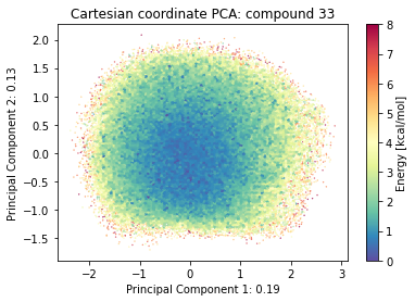
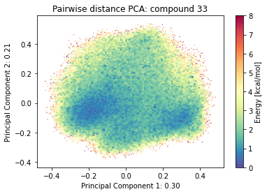
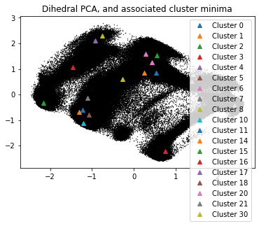
The simulation trajectories contain the positions of all atoms. This high dimensional data (3*N_atoms) is too complicated to analyse by itself. To get a feeling of the potential energy landscape we need to apply some kind of dimensionality reduction. Here, we apply the PCA (Principal Component Analysis) method.
2.9.4.1. Cartesian PCA#
Details about cartesian PCA
t.n_frames
500000
2.9.4.2. Pairwise distances PCA#
2.9.4.3. Dihedral PCA#
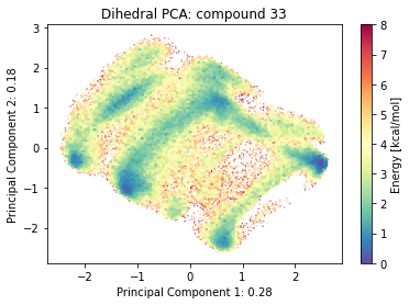
if beta_run:
    # Plot structural digits on top of dPCA
    fig, axs = plt.subplots(2,5, sharex='all', sharey='all')
    fig.set_size_inches(12,8)
    for i in range(10):
        axs.flatten()[i] = src.pca.plot_PCA(reduced_dihedrals, 'dihedral', compound_index, d_weights, 'Energy [kcal/mol]', fig, axs.flatten()[i], cbar_plot='nocbar')
        axs.flatten()[i].scatter(reduced_dihedrals[idxs[i]][:,0], reduced_dihedrals[idxs[i]][:,1], label=values[i], s=0.2, marker=".", color='black')
        axs.flatten()[i].set_title(f"{values[i]}: {motive_percentage[i][1]:.2f}%")
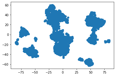
2.9.4.4. TSNE#
# TSNE dimensionality reduction
# TSNE
cluster_stride = plot_stride # 125 previously
dihe = src.dihedrals.getReducedDihedrals(t)
tsne = TSNE(n_components=2, verbose=0, perplexity=50, n_iter=2000, random_state=42)
tsne_results = tsne.fit_transform(dihe[::cluster_stride,:]) # 250
plt.scatter(tsne_results[:,0], tsne_results[:,1])
plt.show()
/biggin/b147/univ4859/research/snakemake_conda/9a8fac97661a24a566a4d6ee98b8d3e7/lib/python3.7/site-packages/sklearn/manifold/_t_sne.py:783: FutureWarning: The default initialization in TSNE will change from 'random' to 'pca' in 1.2.
  FutureWarning,
/biggin/b147/univ4859/research/snakemake_conda/9a8fac97661a24a566a4d6ee98b8d3e7/lib/python3.7/site-packages/sklearn/manifold/_t_sne.py:793: FutureWarning: The default learning rate in TSNE will change from 200.0 to 'auto' in 1.2.
  FutureWarning,
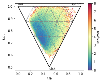
# Shape analysis - principal moments of inertia
inertia_tensor = md.compute_inertia_tensor(t)
principal_moments = np.linalg.eigvalsh(inertia_tensor)
principal_moments
array([[ 46.24272938, 119.02571792, 129.13264031],
       [ 42.74083353, 114.66553182, 129.10689525],
       [ 44.92907934, 114.99417224, 127.74162738],
       ...,
       [ 49.65657075, 105.502946  , 141.1773837 ],
       [ 49.77446746, 110.34543044, 143.66144767],
       [ 48.26291161, 101.73625025, 131.7244535 ]])
# Compute normalized principal moments of inertia
npr1 = principal_moments[:,0] / principal_moments[:,2]
npr2 = principal_moments[:,1] / principal_moments[:,2]
mol_shape = np.stack((npr1, npr2), axis=1)
mol_shape.shape
(500000, 2)
# Reweighting
if snakemake.params.method == "cMD":
    mol_shape_weights = reweight(mol_shape, None, 'noweight')
else:
    weight_data = np.loadtxt(snakemake.input.weights)
    mol_shape_weights = reweight(mol_shape, snakemake.input.weights, 'amdweight_MC', weight_data)
# save
pickle_dump(snakemake.output.NPR_shape_data, mol_shape)
pickle_dump(snakemake.output.NPR_shape_weights, mol_shape_weights)
import matplotlib.tri as tri
x = mol_shape[:,0]
y = mol_shape[:,1]
v= mol_shape_weights
# create a triangulation out of these points
T = tri.Triangulation(x,y)

fig, ax = plt.subplots()
fig.set_size_inches(5,4)

# plot the contour
#plt.tricontourf(x,y,T.triangles,v)
scat = ax.scatter(mol_shape[:,0], mol_shape[:,1], s=0.5, c=mol_shape_weights, cmap='Spectral_r', vmin=0, vmax=8)

# create the grid
corners = np.array([[1, 1], [0.5, 0.5], [0,1]])
triangle = tri.Triangulation(corners[:, 0], corners[:, 1])

# creating the outline
refiner = tri.UniformTriRefiner(triangle)
outline = refiner.refine_triangulation(subdiv=0)

# creating the outline
refiner = tri.UniformTriRefiner(triangle)
trimesh = refiner.refine_triangulation(subdiv=2)

colorbar = fig.colorbar(scat, ax=ax, label="kcal/mol")

#plotting the mesh
ax.triplot(trimesh,'--', color='grey')
ax.triplot(outline,'k-')
ax.set_xlabel(r'$I_{1}/I_{3}$')
ax.set_ylabel('$I_{2}/I_{3}$')
ax.text(0 ,1.01, 'rod')
ax.text(0.85 ,1.01, 'sphere')
ax.text(0.5 ,0.48, 'disk')

fig.savefig(snakemake.output.NPR_shape_plot, dpi=300)
if beta_run:
    # SASA
    sasa = md.shrake_rupley(t)
    total_sasa = sasa.sum(axis=1)
if beta_run:
    plt.plot(t.time, total_sasa)
if beta_run:
    plt.hist(total_sasa)
if beta_run:
    # SASA Reweighting
    if snakemake.params.method == "cMD":
        pmf, distances = src.reweight_1d_pmf(total_sasa, None, 'noweight')
    else:
        pmf, distances = src.reweight_1d_pmf(total_sasa, snakemake.input.weights, 'amdweight_MC')
if beta_run:
    plt.plot(distances[:-1], pmf, label='SASA')
    plt.xlabel(r'SASA ($\AA$)')
    plt.ylabel('PMF (kcal/mol)')
    plt.title(f"Compound {compound_index}")
    plt.savefig(snakemake.output.sasa_plot)
if beta_run:
    weights = np.exp(-1 * pmf / 0.5961)
    weights_norm = weights / np.sum(weights)
    sasa_average = weights_norm * pmf
if beta_run:
    def autocorr(x):
        "Compute an autocorrelation with numpy"
        x = x - np.mean(x)
        result = np.correlate(x, x, mode='full')
        result = result[result.size//2:]
        return result / result[0]

    plt.semilogx(t.time, autocorr(total_sasa))
    plt.xlabel('Time [ps]', size=16)
    plt.ylabel('SASA autocorrelation', size=16)
    plt.show()
#if beta_run:
# Cremer pople analysis
from rdkit import Chem
# load rdkit ref
# Read in pdb file from amber
#mol_ref = Chem.MolFromPDBFile(pdb_amber, removeHs=False, proximityBonding=True) #removeHs=True, proximityBonding=True)
mol_ref = Chem.MolFromMol2File(snakemake.input.ref_mol, removeHs=False,)
mol_ref.RemoveAllConformers()
mol_ref
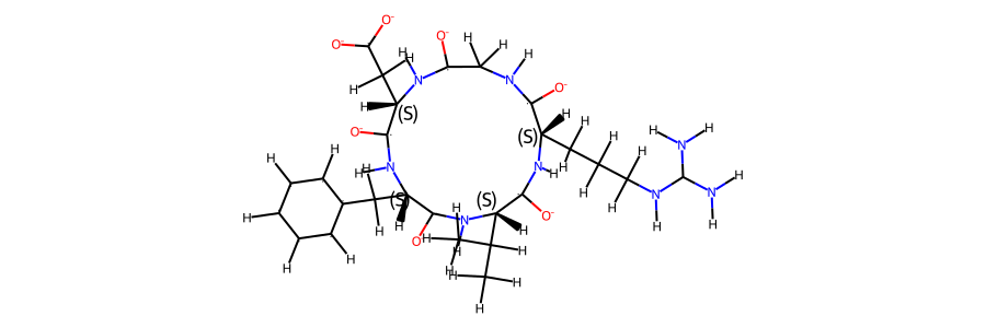
mol_ref.GetNumAtoms() == t.n_atoms
True
import py_rdl
# Get Bond Set
bonds = []
for bond in mol_ref.GetBonds():
    bonds.append((bond.GetBeginAtom().GetIdx(),bond.GetEndAtom().GetIdx()))

cremerpople_store = []

data = py_rdl.Calculator.get_calculated_result(bonds)

ring_length = []
for urf in data.urfs:
    rcs = data.get_relevant_cycles_for_urf(urf)
    for rc in rcs:
        ring_length.append(len(src.Ring_Analysis.Rearrangement(mol_ref, list(rc.nodes))))
max_ring = ring_length.index(max(ring_length))


#for urf in data.urfs:
urf = data.urfs[max_ring]
rcs = data.get_relevant_cycles_for_urf(urf)
for rc in rcs:
    ringloop = src.Ring_Analysis.Rearrangement(mol_ref, list(rc.nodes)) # rearrange the ring atom order
    # src.Ring_Analysis.CTPOrder(mol_ref, list(rc.nodes), n_res=t.n_residues) ## this does not work...
    coord = t.xyz[:,ringloop]
    for i in range(t.n_frames):
        ccoord = src.Ring_Analysis.Translate(coord[i])
        qs, angle = src.Ring_Analysis.GetRingPuckerCoords(ccoord) # get cremer-pople parameters
        qs.extend([abs(x) for x in angle])
        cremerpople_store.append(qs) # flatten tuple/list to just 1d list...
        #coord = np.array([mol0.GetConformer(1).GetAtomPosition(atom) for atom in ringloop]) # get current ring atom coordinates
        #ccoord = RA.Translate(coord) # translate ring with origin as cetner
        #cremerpople = RA.GetRingPuckerCoords(ccoord) # get cremer-pople parameters
cremerpople_store = np.array(cremerpople_store)
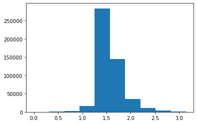
plt.hist(cremerpople_store[:,9])
(array([   297.,    585.,   2136.,  16733., 283961., 145238.,  35883.,
         10541.,   3230.,   1396.]),
 array([7.34978939e-04, 3.14807077e-01, 6.28879176e-01, 9.42951275e-01,
        1.25702337e+00, 1.57109547e+00, 1.88516757e+00, 2.19923967e+00,
        2.51331177e+00, 2.82738387e+00, 3.14145596e+00]),
 <BarContainer object of 10 artists>)
# if beta_run:
#     cremerpople_store = cremerpople_store[1000000:]
from sklearn.decomposition import PCA
from sklearn.preprocessing import normalize
pca = PCA(n_components=2)
pca_input = cremerpople_store.reshape(t.n_frames, len(qs))

#normalize(cremerpople_store.reshape(t.n_frames, len(qs)))


cp_reduced_output = pca.fit_transform(pca_input)

if snakemake.params.method == "cMD":
    cp_weights = reweight(cp_reduced_output, None, 'noweight')
else:
    weight_data = np.loadtxt(snakemake.input.weights)
    weight_data = weight_data[::stride]
    cp_weights = reweight(cp_reduced_output, snakemake.input.weights, 'amdweight_MC', weight_data)

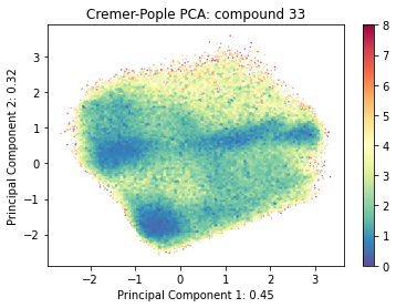
ax = src.pca.plot_PCA(cp_reduced_output, 'CP', compound_index, cp_weights, explained_variance=pca.explained_variance_ratio_[:2])
if multiple:
    src.pca.plot_PCA_citra(cp_reduced_output[cis], cp_reduced_output[trans], 'dihedral', compound_index, label=None, fig=None, ax=None)
pca.explained_variance_ratio_
array([0.4467909 , 0.31815399])
beta_run = False
2.9.4.5. Comparison#
beta_run = True
2.9.5. DBSCAN-Clustering#
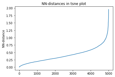
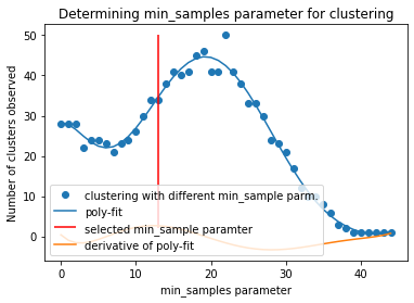
The following section provides details about the performed DBSCAN clustering. Detailed plots about parameter derivation for the clustering are hidden, but can be revealed.
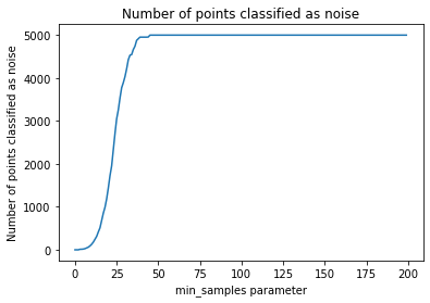
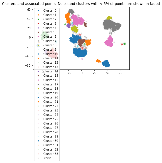
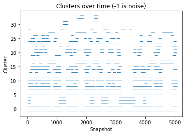
There are 34 clusters
Cluster 0 makes up more than 5% of points. (5.82 % of total points)
Cluster 1 makes up more than 5% of points. (2.54 % of total points)
Cluster 2 makes up more than 5% of points. (5.74 % of total points)
Cluster 3 makes up more than 5% of points. (7.9 % of total points)
Cluster 4 makes up more than 5% of points. (1.0 % of total points)
Cluster 5 makes up more than 5% of points. (3.46 % of total points)
Cluster 6 makes up more than 5% of points. (8.32 % of total points)
Cluster 7 makes up more than 5% of points. (2.42 % of total points)
Cluster 8 makes up more than 5% of points. (2.92 % of total points)
Exlude Cluster 9 is less than 5% of points. (0.38 % of total points)
Cluster 10 makes up more than 5% of points. (9.98 % of total points)
Cluster 11 makes up more than 5% of points. (4.06 % of total points)
Exlude Cluster 12 is less than 5% of points. (0.4 % of total points)
Exlude Cluster 13 is less than 5% of points. (0.44 % of total points)
Cluster 14 makes up more than 5% of points. (1.32 % of total points)
Cluster 15 makes up more than 5% of points. (1.16 % of total points)
Cluster 16 makes up more than 5% of points. (6.859999999999999 % of total points)
Cluster 17 makes up more than 5% of points. (14.24 % of total points)
Cluster 18 makes up more than 5% of points. (1.26 % of total points)
Exlude Cluster 19 is less than 5% of points. (0.32 % of total points)
Cluster 20 makes up more than 5% of points. (4.96 % of total points)
Cluster 21 makes up more than 5% of points. (1.38 % of total points)
Exlude Cluster 22 is less than 5% of points. (0.33999999999999997 % of total points)
Exlude Cluster 23 is less than 5% of points. (0.74 % of total points)
Exlude Cluster 24 is less than 5% of points. (0.45999999999999996 % of total points)
Exlude Cluster 25 is less than 5% of points. (0.33999999999999997 % of total points)
Exlude Cluster 26 is less than 5% of points. (0.26 % of total points)
Exlude Cluster 27 is less than 5% of points. (0.76 % of total points)
Exlude Cluster 28 is less than 5% of points. (0.24 % of total points)
Exlude Cluster 29 is less than 5% of points. (0.8999999999999999 % of total points)
Cluster 30 makes up more than 5% of points. (1.04 % of total points)
Exlude Cluster 31 is less than 5% of points. (0.38 % of total points)
Exlude Cluster 32 is less than 5% of points. (0.9400000000000001 % of total points)
Exlude Cluster 33 is less than 5% of points. (0.45999999999999996 % of total points)
Noise makes up 6.260000000000001 % of total points.
/biggin/b147/univ4859/research/snakemake_conda/9a8fac97661a24a566a4d6ee98b8d3e7/lib/python3.7/site-packages/ipykernel_launcher.py:37: UserWarning: Tight layout not applied. The bottom and top margins cannot be made large enough to accommodate all axes decorations.
/biggin/b147/univ4859/research/snakemake_conda/9a8fac97661a24a566a4d6ee98b8d3e7/lib/python3.7/site-packages/ipykernel_launcher.py:8: UserWarning: Creating legend with loc="best" can be slow with large amounts of data.

/biggin/b147/univ4859/research/snakemake_conda/9a8fac97661a24a566a4d6ee98b8d3e7/lib/python3.7/site-packages/IPython/core/pylabtools.py:151: UserWarning: Creating legend with loc="best" can be slow with large amounts of data.
  fig.canvas.print_figure(bytes_io, **kw)
cluster_traj = t[cluster_index]
cluster_traj.superpose(cluster_traj, 0, atom_indices = cluster_traj.top.select('backbone'))
view = nv.show_mdtraj(cluster_traj)
view
# save rst files from clusters
for idx in cluster_index:
    cluster_full_t = md.load_frame(snakemake.input.traj, idx, top=snakemake.input.top)
    cluster_full_t.save_netcdfrst(f"{snakemake.params.rst_dir}rst_{idx}.rst") #snakemake.output.rst)
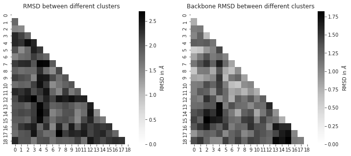
# compute dihedral angles
*_, omega = src.dihedrals.getDihedrals(cluster_traj)
omega_deg = np.abs(np.degrees(omega))
plt.plot(omega_deg)
plt.title(f"Omega angles of different clusters. Compound {compound_index}")
plt.show()
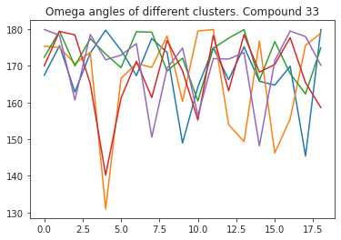
Colors appended..

# cluster NOE statistics....
2.9.6. NOEs#
In the following section, we compute the NOE values for the simulation.
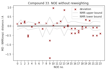
2.9.6.1. NOE without reweighting.#
The following NOE plot is computed via r^-6 averaging. No reweighting is performed. (so unless the simulation is a conventional MD simulation, the following plot is not a valid comparison to experiment.)
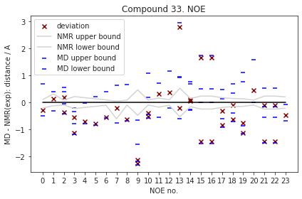
2.9.6.2. Reweighted NOEs#
The following NOE plot was reweighted via a 1d PMF method.
| Atom 1 | Atom 2 | NMR exp | lower bound | upper bound | md | lower | upper | |
|---|---|---|---|---|---|---|---|---|
| 0 | (32,) | (44,) | 2.50 | 2.30 | 2.61 | 2.223813 | 2.013577 | 3.192459 |
| 1 | (1,) | (3,) | 2.55 | 2.43 | 2.87 | 2.684123 | 2.25391 | 2.964648 |
| 2 | (25,) | (27, 28) | 2.35 | 2.26 | 2.44 | 2.543437 | 2.308136 | 2.90923 |
| 2 | (25,) | (27, 28) | 2.35 | 2.26 | 2.44 | 1.982733 | 1.936192 | 2.756192 |
| 3 | (25,) | (27, 28) | 3.10 | 2.88 | 3.32 | 2.543437 | 2.308136 | 2.90923 |
| 3 | (25,) | (27, 28) | 3.10 | 2.88 | 3.32 | 1.982733 | 1.936192 | 2.756192 |
| 4 | (32,) | (34,) | 2.89 | 2.71 | 3.07 | 2.201294 | 2.105565 | 2.881432 |
| 5 | (44,) | (46,) | 2.67 | 2.53 | 2.81 | 1.892169 | 1.839757 | 2.893605 |
| 6 | (64,) | (66,) | 2.40 | 2.30 | 2.50 | 1.858849 | 1.828337 | 2.811764 |
| 7 | (1,) | (66,) | 2.90 | 2.30 | 2.95 | 2.6982 | 2.152701 | 3.545015 |
| 8 | (25,) | (3,) | 2.34 | 2.25 | 2.43 | 1.707773 | 1.673022 | 3.015438 |
| 9 | (32,) | (27, 28) | 4.00 | 3.53 | 4.47 | 1.886019 | 1.833296 | 3.359337 |
| 9 | (32,) | (27, 28) | 4.00 | 3.53 | 4.47 | 1.743923 | 1.700287 | 2.451658 |
| 10 | (32,) | (27, 28) | 2.27 | 2.18 | 2.36 | 1.886019 | 1.833296 | 3.359337 |
| 10 | (32,) | (27, 28) | 2.27 | 2.18 | 2.36 | 1.743923 | 1.700287 | 2.451658 |
| 11 | (44,) | (34,) | 2.85 | 2.68 | 3.02 | 3.177936 | 2.309314 | 3.557197 |
| 12 | (64,) | (46,) | 2.40 | 2.30 | 2.50 | 2.782222 | 2.188323 | 3.555814 |
| 13 | (44,) | (27, 28) | 4.17 | 3.64 | 4.70 | 6.971748 | 5.122754 | 7.111633 |
| 13 | (44,) | (27, 28) | 4.17 | 3.64 | 4.70 | 3.976058 | 3.565023 | 5.108969 |
| 14 | (44,) | (48, 49) | 2.75 | 2.60 | 2.90 | 2.862614 | 2.508124 | 3.444878 |
| 14 | (44,) | (48, 49) | 2.75 | 2.60 | 2.90 | 2.815026 | 2.462447 | 3.513522 |
| 15 | (44,) | (36, 37) | 3.20 | 2.96 | 3.44 | 1.760956 | 1.691228 | 3.70857 |
| 15 | (44,) | (36, 37) | 3.20 | 2.96 | 3.44 | 4.856667 | 3.214991 | 4.930321 |
| 16 | (44,) | (36, 37) | 3.20 | 2.96 | 3.44 | 1.760956 | 1.691228 | 3.70857 |
| 16 | (44,) | (36, 37) | 3.20 | 2.96 | 3.44 | 4.856667 | 3.214991 | 4.930321 |
| 17 | (32,) | (36, 37) | 2.92 | 2.74 | 3.10 | 2.616129 | 2.321569 | 3.402815 |
| 17 | (32,) | (36, 37) | 2.92 | 2.74 | 3.10 | 2.087653 | 1.998107 | 3.053774 |
| 18 | (32,) | (36, 37) | 2.71 | 2.56 | 2.86 | 2.616129 | 2.321569 | 3.402815 |
| 18 | (32,) | (36, 37) | 2.71 | 2.56 | 2.86 | 2.087653 | 1.998107 | 3.053774 |
| 19 | (64,) | (48, 49) | 2.70 | 2.56 | 2.84 | 1.586751 | 1.550094 | 3.812239 |
| 19 | (64,) | (48, 49) | 2.70 | 2.56 | 2.84 | 1.956244 | 1.840696 | 3.469857 |
| 20 | (1,) | (68,) | 2.35 | 2.26 | 2.44 | 2.797285 | 2.351473 | 3.940611 |
| 21 | (1,) | (5, 6) | 3.22 | 2.98 | 3.46 | 1.779399 | 1.737968 | 3.059249 |
| 21 | (1,) | (5, 6) | 3.22 | 2.98 | 3.46 | 3.135034 | 2.673663 | 3.766305 |
| 22 | (1,) | (5, 6) | 3.22 | 2.98 | 3.46 | 1.779399 | 1.737968 | 3.059249 |
| 22 | (1,) | (5, 6) | 3.22 | 2.98 | 3.46 | 3.135034 | 2.673663 | 3.766305 |
| 23 | (66,) | (68,) | 3.08 | 2.87 | 3.29 | 2.606916 | 2.396975 | 3.005951 |
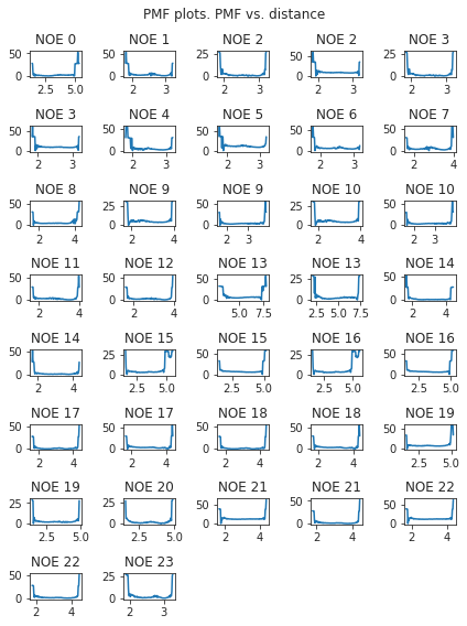
2.9.7. Statistics#
Following, we compute various statistical metrics to evaluate how the simulated NOEs compare to the experimental ones.
def compute_fulfilled_percentage(NOE_df):
    # I: exp_low/exp_high exist
    # exp_low <= md <= exp_high        -> fulfilled
    # md < exp_low OR exp_high < md  -> not fulfilled

    # II: no exp_low:
    #md <= exp_high     -> fulfilled?

    #md > exp_high      -> not fulfilled

    # III: no exp_high:
    #20% of exp value ~ exp_high
    #md < exp_low       -> not fulfilled

    # IV: no exp_low, no exp_high:
    #20% of exp value ~ exp high

    # treat non-existence of lower bound as a lower bound of 0 (ignore / always fulfilled) in previous scripts
    # so this should work for no lower bound available.
    # if there is only bounds, e.g. no NMR exp, this should still work, since the if np.all evaluates to false,
    # and the 'NMR exp' column is not required..

    # upper bound does not exist:
    if np.all(NOE_df["upper bound"] == 0):
        # set higher bound to 20% of experimental value
        high_bound_value = 0.2
        NOE_df["upper bound"] = NOE_df["NMR exp"] + (NOE_df["NMR exp"] * 0.2)


    fulfilled = (NOE_df["md"] <= NOE_df["upper bound"]) & (NOE_df["md"] >= NOE_df["lower bound"])

    return sum(fulfilled) / len(fulfilled)
# % fulfilled
if multiple:
    if len(cis) > CIS_TRANS_CUTOFF:
        # cis
        fulfilled = compute_fulfilled_percentage(NOE_cis_t)
        append = {'stat': 'percentage_fulfilled', 'value': fulfilled, 'up': 0, 'low': 0}
        NOE_stat_cis = NOE_stat_cis.append(append, ignore_index=True)
    if len(trans) > CIS_TRANS_CUTOFF:
        # trans
        fulfilled = compute_fulfilled_percentage(NOE_trans_t)
        append = {'stat': 'percentage_fulfilled', 'value': fulfilled, 'up': 0, 'low': 0}
        NOE_stat_trans = NOE_stat_trans.append(append, ignore_index=True)
else:
    fulfilled = compute_fulfilled_percentage(NOE_test)

    append = {'stat': 'percentage_fulfilled', 'value': fulfilled, 'up': 0, 'low': 0}
    NOE_stats = NOE_stats.append(append, ignore_index=True)
# is the mean deviation significantly different than 0? if pvalue < 5% -> yes! We want: no! (does not deviate from exp. values)
if multiple:
    if len(cis) > CIS_TRANS_CUTOFF:
        print(stats.ttest_1samp(NOE_cis_t['dev'], 0.0))
    if len(trans) > CIS_TRANS_CUTOFF:
        print(stats.ttest_1samp(NOE_trans_t['dev'], 0.0))
else:
    print(stats.ttest_1samp(NOE_test['dev'], 0.0))
Ttest_1sampResult(statistic=-3.1539001111776903, pvalue=0.004441068913561296)
if multiple:
    if len(cis) > CIS_TRANS_CUTOFF:
        print(stats.describe(NOE_cis_t['dev']))
    if len(trans) > CIS_TRANS_CUTOFF:
        print(stats.describe(NOE_trans_t['dev']))
else:
    print(stats.describe(NOE_test['dev']))
DescribeResult(nobs=24, minmax=(-2.113980917934902, 0.44728502406711357), mean=-0.39495594751191304, variance=0.3763679981041342, skewness=-1.058478701188106, kurtosis=1.0263018147926788)
NOE statistics:
| stat | value | up | low | |
|---|---|---|---|---|
| 0 | MAE | 0.524125 | 0.738091 | 0.346424 |
| 1 | MSE | -0.394956 | -0.166937 | 0.000000 |
| 2 | RMSD | 0.718802 | 0.983416 | 0.431724 |
| 3 | pearsonr | 0.339355 | 0.770992 | 0.000000 |
| 4 | kendalltau | 0.173113 | 0.520252 | 0.000000 |
| 5 | chisq | 3.838673 | 6.626588 | 1.646457 |
| 6 | percentage_fulfilled | 0.291667 | 0.000000 | 0.000000 |
# # NOE_test
# NOE_path = snakemake.input.noe

# max_populated_cluster_idx = np.argmax(cluster_percentage)
# max_populated_cluster = cluster_traj[max_populated_cluster_idx]
# max_populated_cluster_original_traj_idx = cluster_index[max_populated_cluster_idx]

# NOE = src.noe.read_NOE(NOE_path)
# if multiple:
#     NOE_trans, NOE_cis = NOE
#     NOE_cis_dict = NOE_cis.to_dict(orient='index')
#     NOE_trans_dict = NOE_trans.to_dict(orient='index')
# else:
#     NOE_dict = NOE.to_dict(orient='index')
# current_cluster = cluster_traj[i]
# if multiple:
#     if max_populated_cluster_original_traj_idx in cis:
#         #print("cis")
#         NOE_dict = NOE_cis_dict
#         NOE = NOE_cis
#     else:
#         #print("trans!")
#         NOE_dict = NOE_trans_dict
#         NOE = NOE_trans
# else:
#     axs[i,2].set_title(f"Cluster {k}")
# NOE['md'],_,_2,NOE_dist, _3 = src.noe.compute_NOE_mdtraj(NOE_dict, max_populated_cluster)
# # Deal with ambigous NOEs
# NOE = NOE.explode('md')
# # and ambigous/multiple values
# NOE = NOE.explode('NMR exp')
if multiple:
    NOE_stats_keys = ['cis', 'trans']
    differentiation = {'cis':cis, 'trans':trans}
else:
    NOE_stats_keys = ['single']
n_cluster_traj = {}
n_cluster_percentage = {}
n_cluster_index = {}
for k in NOE_stats_keys:
    if multiple:
        cluster_in_x = np.in1d(cluster_index, differentiation[k])
#         np.arange()
    else:
        cluster_in_x = np.ones((len(cluster_index)), dtype=bool)
    cluster_in_x = np.arange(0, len(cluster_index))[cluster_in_x]
    n_cluster_traj[k] = cluster_traj[cluster_in_x]
    n_cluster_percentage[k] = np.array(cluster_percentage)[cluster_in_x]
    n_cluster_index[k] = np.array(cluster_index)[cluster_in_x]
cluster_traj = n_cluster_traj
cluster_percentage = n_cluster_percentage
cluster_index = n_cluster_index
cluster_percentage
{'single': array([0.0582, 0.0254, 0.0574, 0.079 , 0.01  , 0.0346, 0.0832, 0.0242,
        0.0292, 0.0998, 0.0406, 0.0132, 0.0116, 0.0686, 0.1424, 0.0126,
        0.0496, 0.0138, 0.0104])}
# NOE_stat_combined
NOE_dict = {}
NOE = src.noe.read_NOE(NOE_path)
NOE_n = {}
if multiple:
    NOE_trans, NOE_cis = NOE
    NOE_n['cis'] = NOE_cis
    NOE_n['trans'] = NOE_trans
    NOE_dict['cis'] = NOE_cis.to_dict(orient='index')
    NOE_dict['trans'] = NOE_trans.to_dict(orient='index')
else:
    NOE_dict['single'] = NOE.to_dict(orient='index')
    NOE_n['single'] = NOE


for k in NOE_stats_keys:
    # max. populated cluster
    # NOE = NOE_n.copy()
    max_populated_cluster_idx = np.argmax(cluster_percentage[k])
    max_populated_cluster = cluster_traj[k][max_populated_cluster_idx]
    NOE_n[k]['md'],*_ = src.noe.compute_NOE_mdtraj(NOE_dict[k], max_populated_cluster)
    # Deal with ambigous NOEs
    NOE_n[k] = NOE_n[k].explode('md')
    # and ambigous/multiple values
    NOE_n[k] = NOE_n[k].explode('NMR exp')

    # Remove duplicate values (keep value closest to experimental value)
    NOE_test = NOE_n[k]
    if (NOE_test['NMR exp'].to_numpy() == 0).all():
        # if all exp values are 0: take middle between upper / lower bound as reference value
        NOE_test['NMR exp'] = (NOE_test['upper bound'] + NOE_test['lower bound']) * 0.5
    NOE_test['dev'] = NOE_test['md'] - np.abs(NOE_test['NMR exp'])
    NOE_test['abs_dev'] = np.abs(NOE_test['md'] - np.abs(NOE_test['NMR exp']))

    NOE_test = NOE_test.sort_values('abs_dev',ascending=True)
    NOE_test.index = NOE_test.index.astype(int)
    NOE_test = NOE_test[~NOE_test.index.duplicated(keep='first')].sort_index(kind='mergesort')

    # drop NaN values:
    NOE_test = NOE_test.dropna()
    # Compute metrics now
    # Compute NOE statistics, since no bootstrap necessary, do a single iteration.. TODO: could clean this up further to pass 0, then just return the value...
    RMSD,*_ = src.stats.compute_RMSD(NOE_test['NMR exp'], NOE_test['md'], n_bootstrap=1)
    MAE, *_ = src.stats.compute_MAE(NOE_test['NMR exp'], NOE_test['md'], n_bootstrap=1)
    MSE,  *_ = src.stats.compute_MSE(NOE_test['dev'], n_bootstrap=1)
    fulfil = src.stats.compute_fulfilled_percentage(NOE_test)
    #insert values
    values = [MAE,MSE,RMSD,None,None,None,fulfil]
    n_NOE_stat[k].insert(4, "most-populated-1", values)
#     MAE
#     MSE
#     RMSD
#     pearsonr
#     kendalltau
#     chisq
#     percentage_fulfilled
for k in NOE_stats_keys:
    display(n_NOE_stat[k])
    # convert df to dict for export
    n_NOE_stat[k] = n_NOE_stat[k].to_dict()
# Save
src.utils.json_dump(snakemake.output.noe_stats, n_NOE_stat)
| stat | value | up | low | most-populated-1 | |
|---|---|---|---|---|---|
| 0 | MAE | 0.524125 | 0.738091 | 0.346424 | 0.345824 |
| 1 | MSE | -0.394956 | -0.166937 | 0.000000 | 0.127284 |
| 2 | RMSD | 0.718802 | 0.983416 | 0.431724 | 0.483685 |
| 3 | pearsonr | 0.339355 | 0.770992 | 0.000000 | NaN |
| 4 | kendalltau | 0.173113 | 0.520252 | 0.000000 | NaN |
| 5 | chisq | 3.838673 | 6.626588 | 1.646457 | NaN |
| 6 | percentage_fulfilled | 0.291667 | 0.000000 | 0.000000 | 0.375000 |
# # Cluster NOE metrics
# if multiple:
#     if len(cis) > CIS_TRANS_CUTOFF:
#         # cis
#         fulfilled = compute_fulfilled_percentage(NOE_cis_t)
#         append = {'stat': 'percentage_fulfilled', 'value': fulfilled, 'up': 0, 'low': 0}
#         NOE_stat_cis = NOE_stat_cis.append(append, ignore_index=True)
#     if len(trans) > CIS_TRANS_CUTOFF:
#         # trans
#         fulfilled = compute_fulfilled_percentage(NOE_trans_t)
#         append = {'stat': 'percentage_fulfilled', 'value': fulfilled, 'up': 0, 'low': 0}
#         NOE_stat_trans = NOE_stat_trans.append(append, ignore_index=True)
# else:
#     fulfilled = compute_fulfilled_percentage(NOE_test)

#     append = {'stat': 'percentage_fulfilled', 'value': fulfilled, 'up': 0, 'low': 0}
#     NOE_stats = NOE_stats.append(append, ignore_index=True)
# NOE_stats = {}

# if multiple:
#     NOE_stats_keys = ['cis', 'trans']
# else:
#     NOE_stats_keys = ['single']

# for k in NOE_stats_keys:
# #     NOE_stats[k] = pd.DataFrame(columns=['stat', 'value', 'up', 'low'])
#     NOE_stats[k] = NOE_stats[k].insert(3, "most-populated-1", values)
# for k in NOE_stats_keys:
# #     MAE =
# #     MSE =
# #     RMSD =
# #     pearsonr =
# #     kendalltau =
# #     chisq =
# #     percentage_fulfilled =

#     NOE_stats[k].append()
# compute_fulfilled_percentage(NOE)
# compute_RMSD(NOE['NMR exp'], NOE['md'])[0]
print('Done')
Done
