Analysis Notebook
Contents
2.14. Analysis Notebook#
A copy of this notebook is run to analyse the molecular dynamics simulations. The type of MD simulation is specified in the Snakemake rule as a parameter, such that it is accessible via: snakemake.params.method.
There are various additional analysis steps, that are included in the notebook,
but are not part of the paper. To turn these on, set the beta_run parameter to True.
There are also some commented out lines in the notebook. These are mainly for the purpose of debugging. Some of them are for interactively exploring the 3d structure of the system. These don’t work as part of the automated snakemake workflow, but can be enabled when running a notebook interactively.
#Check if we should use shortened trajectories for analysis.
if snakemake.config["shortened"]:
    print("Using shortened trajectories and dihedrals. This only works if these were created previously!")
    if not (os.path.exists(snakemake.params.traj_short)
            and os.path.exists(snakemake.params.dihedrals_short)
            and os.path.exists(snakemake.params.dPCA_weights_MC_short)
            and os.path.exists(snakemake.params.weights_short)
           ):
        raise FileNotFoundError("Shortened trajectories and dihedrals files do not exist, but config value is set to use shortened files! Switch off the use of shortenend files and first analyse this simulation using the full trajectory!")
    else:
        use_shortened = True
else:
    use_shortened = False
# use_shortened = False
# Turn on for development
%load_ext autoreload
%autoreload 2
# Set stride to make prelim. analysis faster. for production, use 1 (use all MD frames)
stride = int(snakemake.config["stride"])
print(f"Using stride {stride} to analyse MD simulations.")
# Perform additional analysis steps (e.g. compute structural digits)
beta_run = False

# Analysing compound
compound_index = int(snakemake.wildcards.compound_dir)
simtime = float(snakemake.wildcards.time)

# Storage
final_figure_axs = []
Using stride 1 to analyse MD simulations.
2.14.1. Compound details#
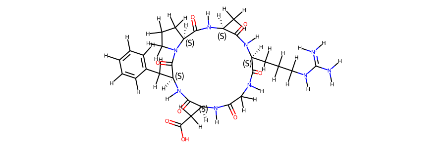
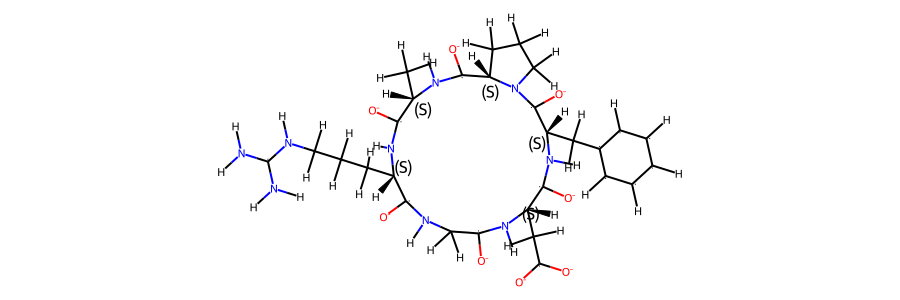
This notebook refers to compound 50.
# TODO: show a 2d image of the molecule, and a 3d structure via py3dmol!
# also put sequence here.
According to the literature reference, there are two distinct structures in solution.
2.14.2. Simulation details#
# TODO: change notebook that it supports use of a shortened trajectory file
# Stereo check 1-frame trajectory to tmp-pdb file
t_stereo_check = topo.restrict_atoms(topo.topology.select("protein or resname ASH"))
tf = tempfile.NamedTemporaryFile(delete=False)
# tf.name
t_stereo_check.save_pdb(tf.name)
# Get reference mol
mol_ref = Chem.MolFromMol2File(
    snakemake.input.ref_mol,
    removeHs=False,
)

# Get 1st frame pdb from tempfile
post_eq_mol = Chem.MolFromPDBFile(
    tf.name,
    removeHs=False,
    sanitize=False,
)

# could compare smiles to automate the stereo-check. Problem: mol2 reference file has wrong bond orders
# (amber does not write those correctly). The ref-pdb file cannot be read b/c geometry is not optimized.
# This leads to funky valences in rdkit. The post-eq pdb file reads fine but then charges etc. dont match
# with the reference (b/c of wrong bond orders). But can manually check that all stereocentres are correct (below)
Chem.CanonSmiles(Chem.MolToSmiles(post_eq_mol)) == Chem.CanonSmiles(
    Chem.MolToSmiles(mol_ref)
)
False
post_eq_mol.RemoveAllConformers()
post_eq_mol
mol_ref.RemoveAllConformers()
mol_ref
The simulation type is cMD, 2000 ns. The simulation was performed in H2O.
There are a total of 500000 frames available to analyse.
# Create a short trajectory & weights if working with the full trajectory
if not use_shortened:
    # determine stride to get 10k frames:
    stride_short = int(t.n_frames / 10000)
    if stride_short == 0:
        stride_short = 1

    # save short trajectory to file
    t[::stride_short].save_netcdf(snakemake.params.traj_short)

    # load weights for GaMD
    if snakemake.params.method == "GaMD":
        weight_data = np.loadtxt(snakemake.input.weights)
        weight_data = weight_data[::stride]
        #create shortened weights
        np.savetxt(snakemake.params.weights_short, weight_data[::stride_short])
else:
    # load shortened weights for GaMD
    if snakemake.params.method == "GaMD":
        weight_data = np.loadtxt(snakemake.params.weights_short)

# this determines a cutoff for when we consider cis/trans conformers separately.
# only relevant if 2 sets of NOE values present.
# t.n_frames / 1000 -> 0.1% of frames need to be cis/trans to consider both forms.
CIS_TRANS_CUTOFF = int(t.n_frames / 1000)
However, for some of the analysis steps below, only 1% of these frames have been used to ensure better rendering in the browser.
2.14.3. Convergence of the simulation#
2.14.3.1. RMSD#
To check for convergence of the simulation, we can look at the root mean squared deviation of the atomic positions over the course of the simulation.
2.14.3.2. Dihedral angles#
# Plot ramachandran plot for each amino acid
if beta_run:
    fig, axs = plt.subplots(int(np.ceil(len(phi.T) / 5)), 5, sharex="all", sharey="all")
    fig.set_size_inches(16, 4)
    motives = []
    i = 0
    for phi_i, psi_i in zip(np.degrees(phi.T), np.degrees(psi.T)):
        weights_phi_psi = reweight(
            np.column_stack((phi_i, psi_i)),
            None,
            "amdweight_MC",
            weight_data,
        )
        axs.flatten()[i].scatter(
            phi_i, psi_i, s=0.5, c=weights_phi_psi, vmin=0, vmax=8, cmap="Spectral_r"
        )
        axs.flatten()[i].set_title(i)
        motives.append(src.dihedrals.miao_ramachandran(phi_i, psi_i))
        i += 1
    fig.show()
if beta_run:
    # compute most common motives
    combined_motives = np.column_stack((motives))
    combined_motives = ["".join(test) for test in combined_motives]
    from collections import Counter

    c = Counter(combined_motives)
    motive_percentage = [
        (i, c[i] / len(combined_motives) * 100.0) for i, count in c.most_common()
    ]
    # 10 most common motives and percentage of frames
    print(motive_percentage[:10])
if beta_run:
    # Get indicies of most common motives
    combined_motives = np.array(combined_motives)
    idxs = []
    values = [i[0] for i in c.most_common(10)]
    for i, v in enumerate(values):
        idxs.append(np.where(combined_motives == v)[0])
2.14.4. Dimensionality Reductions#
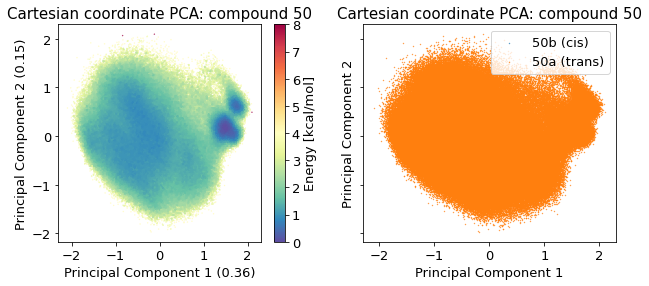
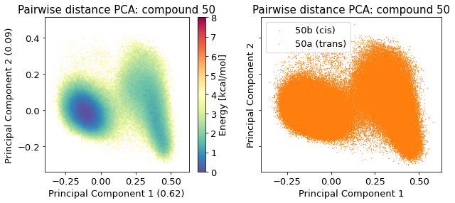
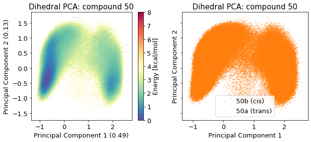
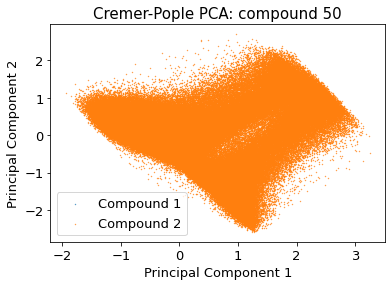
The simulation trajectories contain the positions of all atoms. This high dimensional data (3*N_atoms) is too complicated to analyse by itself. To get a feeling of the potential energy landscape we need to apply some kind of dimensionality reduction. Here, we apply the PCA (Principal Component Analysis) method.
2.14.4.1. Cartesian PCA#
Details about cartesian PCA
/biggin/b147/univ4859/research/snakemake_conda/b998fbb8f687250126238eb7f5e2e52c/lib/python3.7/site-packages/IPython/core/pylabtools.py:151: UserWarning: Creating legend with loc="best" can be slow with large amounts of data.
  fig.canvas.print_figure(bytes_io, **kw)
2.14.4.2. Pairwise distances PCA#
/biggin/b147/univ4859/research/snakemake_conda/b998fbb8f687250126238eb7f5e2e52c/lib/python3.7/site-packages/IPython/core/pylabtools.py:151: UserWarning: Creating legend with loc="best" can be slow with large amounts of data.
  fig.canvas.print_figure(bytes_io, **kw)
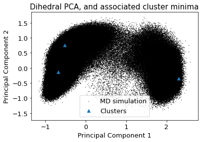
2.14.4.3. Dihedral PCA#
/biggin/b147/univ4859/research/snakemake_conda/b998fbb8f687250126238eb7f5e2e52c/lib/python3.7/site-packages/ipykernel_launcher.py:41: UserWarning: Creating legend with loc="best" can be slow with large amounts of data.
/biggin/b147/univ4859/research/snakemake_conda/b998fbb8f687250126238eb7f5e2e52c/lib/python3.7/site-packages/svgutils/transform.py:425: UserWarning: Creating legend with loc="best" can be slow with large amounts of data.
  fig.savefig(fid, format="svg", **savefig_kw)
/biggin/b147/univ4859/research/snakemake_conda/b998fbb8f687250126238eb7f5e2e52c/lib/python3.7/site-packages/IPython/core/pylabtools.py:151: UserWarning: Creating legend with loc="best" can be slow with large amounts of data.
  fig.canvas.print_figure(bytes_io, **kw)
# pos = reduced_dihedrals
# src.utils.link_ngl_wdgt_to_ax_pos(ax, pos, v)
# v

# phi, psi, omega = src.dihedrals.getDihedrals(t[95852])
# print(np.mean(np.degrees(phi), axis=0), np.mean(np.degrees(psi), axis=0), np.mean(np.degrees(omega), axis=0))
if beta_run:
    # Plot structural digits on top of dPCA
    fig, axs = plt.subplots(2, 5, sharex="all", sharey="all")
    fig.set_size_inches(12, 8)
    for i in range(10):
        axs.flatten()[i] = src.pca.plot_PCA(
            reduced_dihedrals,
            "dihedral",
            compound_index,
            d_weights,
            "Energy [kcal/mol]",
            fig,
            axs.flatten()[i],
            cbar_plot="nocbar",
            explained_variance=pca_d.explained_variance_ratio_[:2],
        )
        axs.flatten()[i].scatter(
            reduced_dihedrals[idxs[i]][:, 0],
            reduced_dihedrals[idxs[i]][:, 1],
            label=values[i],
            s=0.2,
            marker=".",
            color="black",
        )
        axs.flatten()[i].set_title(f"{values[i]}: {motive_percentage[i][1]:.2f}%")
    fig.tight_layout()
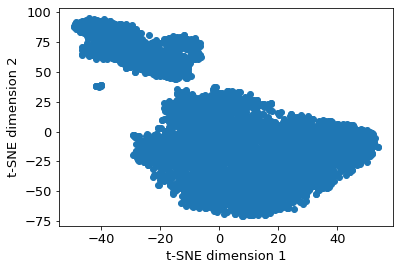
2.14.4.4. TSNE#
# TSNE dimensionality reduction
# TSNE
cluster_stride = plot_stride  # 125 previously
dihe = src.dihedrals.getReducedDihedrals(t)
tsne = TSNE(n_components=2, verbose=0, perplexity=50, n_iter=2000, random_state=42)
tsne_results = tsne.fit_transform(dihe[::cluster_stride, :])  # 250
plt.scatter(tsne_results[:, 0], tsne_results[:, 1])
plt.xlabel("t-SNE dimension 1")
plt.ylabel("t-SNE dimension 2")
plt.show()
/biggin/b147/univ4859/research/snakemake_conda/b998fbb8f687250126238eb7f5e2e52c/lib/python3.7/site-packages/sklearn/manifold/_t_sne.py:783: FutureWarning: The default initialization in TSNE will change from 'random' to 'pca' in 1.2.
  FutureWarning,
/biggin/b147/univ4859/research/snakemake_conda/b998fbb8f687250126238eb7f5e2e52c/lib/python3.7/site-packages/sklearn/manifold/_t_sne.py:793: FutureWarning: The default learning rate in TSNE will change from 200.0 to 'auto' in 1.2.
  FutureWarning,
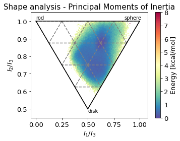
2.14.4.5. Shape analysis - principal moments of inertia#
inertia_tensor = md.compute_inertia_tensor(t)
principal_moments = np.linalg.eigvalsh(inertia_tensor)

# Compute normalized principal moments of inertia
npr1 = principal_moments[:, 0] / principal_moments[:, 2]
npr2 = principal_moments[:, 1] / principal_moments[:, 2]
mol_shape = np.stack((npr1, npr2), axis=1)

# Reweighting
if snakemake.params.method == "cMD":
    mol_shape_weights = reweight(mol_shape, None, "noweight")
else:
    mol_shape_weights = reweight(
        mol_shape, None, "amdweight_MC", weight_data
    )

# save
pickle_dump(snakemake.output.NPR_shape_data, mol_shape)
pickle_dump(snakemake.output.NPR_shape_weights, mol_shape_weights)
# Plot
x = mol_shape[:, 0]
y = mol_shape[:, 1]
v = mol_shape_weights
# create a triangulation out of these points
T = tri.Triangulation(x, y)

fig, ax = plt.subplots()
fig.set_size_inches(5, 4)

# plot the contour
# plt.tricontourf(x,y,T.triangles,v)
scat = ax.scatter(
    mol_shape[:, 0],
    mol_shape[:, 1],
    s=0.5,
    c=mol_shape_weights,
    cmap="Spectral_r",
    vmin=0,
    vmax=8,
    rasterized=True,
)

# create the grid
corners = np.array([[1, 1], [0.5, 0.5], [0, 1]])
triangle = tri.Triangulation(corners[:, 0], corners[:, 1])

# creating the outline
refiner = tri.UniformTriRefiner(triangle)
outline = refiner.refine_triangulation(subdiv=0)

# creating the outline
refiner = tri.UniformTriRefiner(triangle)
trimesh = refiner.refine_triangulation(subdiv=2)

colorbar = fig.colorbar(scat, ax=ax, label="Energy [kcal/mol]")

# plotting the mesh
ax.triplot(trimesh, "--", color="grey")
ax.triplot(outline, "k-")
ax.set_xlabel(r"$I_{1}/I_{3}$")
ax.set_ylabel("$I_{2}/I_{3}$")
ax.text(0, 1.01, "rod")
ax.text(0.85, 1.01, "sphere")
ax.text(0.5, 0.48, "disk")
ax.set_ylim(0.45, 1.05)
ax.set_xlim(-0.05, 1.08)
ax.set_title('Shape analysis - Principal Moments of Inertia')

fig.tight_layout()
fig.savefig(snakemake.output.NPR_shape_plot, dpi=300)
final_figure_axs.append(sg.from_mpl(fig, savefig_kw={"dpi": 300}))
if beta_run:
    # SASA
    sasa = md.shrake_rupley(t)
    total_sasa = sasa.sum(axis=1)
if beta_run:
    x = [x / len(total_sasa) * simtime for x in range(0, len(total_sasa))]
    plt.plot(x, total_sasa)
    plt.xlabel("Simulation time [ns]")
    plt.ylabel("Total SASA [(nm)^2]")
if beta_run:
    plt.hist(total_sasa)
    plt.ylabel("Count")
    plt.xlabel("Total SASA [(nm)^2]")
if beta_run:
    # SASA Reweighting
    if snakemake.params.method == "cMD":
        pmf, distances = src.reweight_1d_pmf(total_sasa, None, "noweight")
    else:
        pmf, distances = src.reweight_1d_pmf(
            total_sasa, None, "amdweight_MC"
        )
    # Plot
    plt.plot(distances[:-1], pmf, label="SASA")
    plt.xlabel(r"SASA ($\AA$)")
    plt.ylabel("PMF (kcal/mol)")
    plt.title(f"Compound {compound_index}")
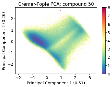
2.14.4.6. Cremer pople analysis#
from rdkit import Chem
import py_rdl

# load topology reference
# mol_ref = Chem.MolFromPDBFile(pdb_amber, removeHs=False, proximityBonding=True) #removeHs=True, proximityBonding=True)
mol_ref = Chem.MolFromMol2File(
    snakemake.input.ref_mol,
    removeHs=False,
)
mol_ref.RemoveAllConformers()
mol_ref

mol_ref.GetNumAtoms() == t.n_atoms
True
# Get Bond Set
bonds = []
for bond in mol_ref.GetBonds():
    bonds.append((bond.GetBeginAtom().GetIdx(), bond.GetEndAtom().GetIdx()))

cremerpople_store = []

data = py_rdl.Calculator.get_calculated_result(bonds)

ring_length = []
for urf in data.urfs:
    rcs = data.get_relevant_cycles_for_urf(urf)
    for rc in rcs:
        ring_length.append(
            len(src.Ring_Analysis.Rearrangement(mol_ref, list(rc.nodes)))
        )
max_ring = ring_length.index(max(ring_length))


# for urf in data.urfs:
urf = data.urfs[max_ring]
rcs = data.get_relevant_cycles_for_urf(urf)
for rc in rcs:
    ringloop = src.Ring_Analysis.Rearrangement(
        mol_ref, list(rc.nodes)
    )  # rearrange the ring atom order
    # src.Ring_Analysis.CTPOrder(mol_ref, list(rc.nodes), n_res=t.n_residues) ## this does not work...
    coord = t.xyz[:, ringloop]
    for i in range(t.n_frames):
        ccoord = src.Ring_Analysis.Translate(coord[i])
        qs, angle = src.Ring_Analysis.GetRingPuckerCoords(
            ccoord
        )  # get cremer-pople parameters
        qs.extend([abs(x) for x in angle])
        cremerpople_store.append(qs)  # flatten tuple/list to just 1d list...
        # coord = np.array([mol0.GetConformer(1).GetAtomPosition(atom) for atom in ringloop]) # get current ring atom coordinates
        # ccoord = RA.Translate(coord) # translate ring with origin as cetner
        # cremerpople = RA.GetRingPuckerCoords(ccoord) # get cremer-pople parameters
cremerpople_store = np.array(cremerpople_store)
# plt.hist(cremerpople_store[:,9])
# if beta_run:
#     cremerpople_store = cremerpople_store[1000000:]
from sklearn.decomposition import PCA
from sklearn.preprocessing import normalize

pca = PCA(n_components=2)
pca_input = cremerpople_store.reshape(t.n_frames, len(qs))

# normalize(cremerpople_store.reshape(t.n_frames, len(qs)))

cp_reduced_output = pca.fit_transform(pca_input)

if snakemake.params.method == "cMD":
    cp_weights = reweight(cp_reduced_output, None, "noweight")
else:
    cp_weights = reweight(
        cp_reduced_output, None, "amdweight_MC", weight_data
    )

ax = src.pca.plot_PCA(
    cp_reduced_output,
    "CP",
    compound_index,
    cp_weights,
    explained_variance=pca.explained_variance_ratio_[:2],
)

if multiple:
    src.pca.plot_PCA_citra(
        cp_reduced_output[cis],
        cp_reduced_output[trans],
        "CP",
        compound_index,
        label=None,
        fig=None,
        ax=None,
    )
/biggin/b147/univ4859/research/snakemake_conda/b998fbb8f687250126238eb7f5e2e52c/lib/python3.7/site-packages/IPython/core/pylabtools.py:151: UserWarning: Creating legend with loc="best" can be slow with large amounts of data.
  fig.canvas.print_figure(bytes_io, **kw)
2.14.4.7. Comparison#
beta_run = True
2.14.5. DBSCAN-Clustering#
The following section provides details about the performed DBSCAN clustering. Detailed plots about parameter derivation for the clustering are hidden, but can be revealed.
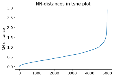
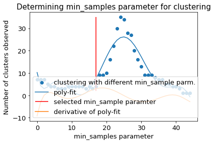
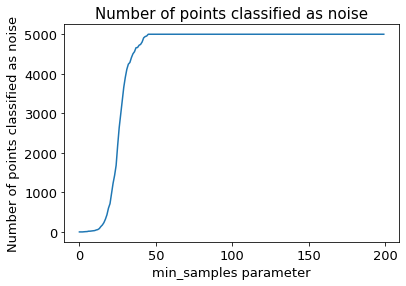
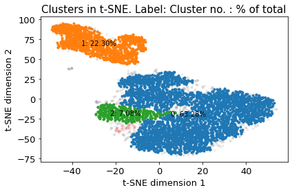
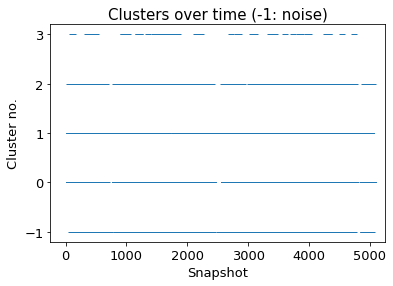
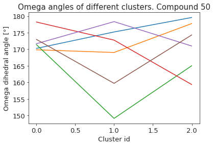
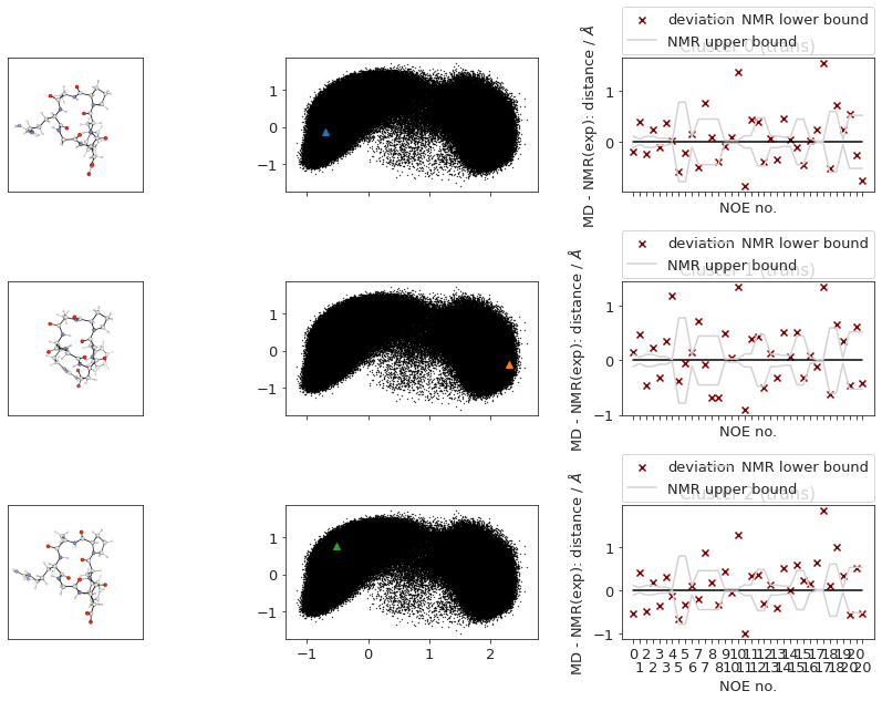
There are 4 clusters
Cluster 0 makes up more than 1.0% of points. (63.28 % of total points)
Cluster 1 makes up more than 1.0% of points. (22.30 % of total points)
Cluster 2 makes up more than 1.0% of points. (7.08 % of total points)
Exlude Cluster 3 is less than 1.0% of points. (0.90 % of total points)
Noise makes up 6.44 % of total points.
/biggin/b147/univ4859/research/snakemake_conda/b998fbb8f687250126238eb7f5e2e52c/lib/python3.7/site-packages/ipykernel_launcher.py:28: UserWarning: Creating legend with loc="best" can be slow with large amounts of data.
/biggin/b147/univ4859/research/snakemake_conda/b998fbb8f687250126238eb7f5e2e52c/lib/python3.7/site-packages/svgutils/transform.py:425: UserWarning: Creating legend with loc="best" can be slow with large amounts of data.
  fig.savefig(fid, format="svg", **savefig_kw)
/biggin/b147/univ4859/research/snakemake_conda/b998fbb8f687250126238eb7f5e2e52c/lib/python3.7/site-packages/IPython/core/pylabtools.py:151: UserWarning: Creating legend with loc="best" can be slow with large amounts of data.
  fig.canvas.print_figure(bytes_io, **kw)
cluster_traj = t[cluster_index]
cluster_traj.superpose(
    cluster_traj, 0, atom_indices=cluster_traj.top.select("backbone")
)
view = nv.show_mdtraj(cluster_traj)
view
# save rst files from clusters, account for GaMD equilibration. Does not work with stride.
cluster_full_store = md.load_frame(snakemake.input.traj, cluster_index[0] + frames_start, top=snakemake.input.top)
for idx in cluster_index:
    cluster_full_t = md.load_frame(snakemake.input.traj, idx, top=snakemake.input.top)
    cluster_full_t.save_netcdfrst(
        f"{snakemake.params.rst_dir}rst_{idx}.rst"
    )  # snakemake.output.rst)
    cluster_full_store = cluster_full_store.join(cluster_full_t, discard_overlapping_frames=True)
cluster_full_store.superpose(
    cluster_full_store, 0, atom_indices=cluster_full_t.top.select("backbone")
)
cluster_full_store.save_pdb(snakemake.output.cluster_solvated)
# hbonds = md.baker_hubbard(t, periodic=True, exclude_water=True, freq=0.2)
# # label = lambda hbond : '%s -- %s' % (t.topology.atom(hbond[0]), t.topology.atom(hbond[2]))
# for hbond in hbonds:
#     print(label(hbond))
# # len(hbonds)
# view2 = nv.show_mdtraj(cluster_full_store, )
# view2.add_representation('licorice', selection="protein")
# view.add_contact(hydrogen_bond=True)
# view2
# compute dihedral angles
*_, omega = src.dihedrals.getDihedrals(cluster_traj)
omega_deg = np.abs(np.degrees(omega))
plt.plot(omega_deg)
plt.title(f"Omega angles of different clusters. Compound {compound_index}")
plt.xlabel("Cluster id")
plt.ylabel("Omega dihedral angle [°]")
plt.show()
# TODO? cluster NOE statistics....
2.14.6. NOEs#
In the following section, we compute the NOE values for the simulation.
2.14.6.1. NOE without reweighting.#
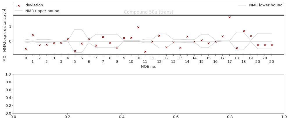
The following NOE plot is computed via r^-6 averaging. No reweighting is performed. (so unless the simulation is a conventional MD simulation, the following plot is not a valid comparison to experiment.)
Cis skipped because no frames are cis.
2.14.6.2. Reweighted NOEs#
The following NOE plot was reweighted via a 1d PMF method.
cMD - no reweighted NOEs performed.
print(plt.rcParams.get('figure.figsize'))
[6.0, 4.0]
(   Atom 1        Atom 2  NMR exp  lower bound  upper bound  \
 0    (1,)         (78,)      0.0         2.77         3.00
 1    (1,)          (3,)      0.0         2.43         2.54
 2    (3,)        (5, 6)      0.0         2.71         2.93
 3    (3,)        (5, 6)      0.0         2.61         2.75
 4   (25,)          (3,)      0.0         2.14         2.18
 5   (25,)      (27, 28)      0.0         2.22         3.79
 6   (32,)         (34,)      0.0         2.66         2.87
 7   (32,)      (36, 37)      0.0         2.40         3.30
 8   (34,)      (36, 37)      0.0         2.42         3.32
 9   (44,)         (32,)      0.0         2.34         2.40
 10  (44,)      (48, 49)      0.0         2.29         2.35
 11  (44,)      (48, 49)      0.0         3.15         3.39
 12  (46,)      (65, 66)      0.0         2.08         3.03
 13  (46,)      (48, 49)      0.0         2.82         3.05
 14  (46,)      (48, 49)      0.0         2.45         2.63
 15  (78,)      (48, 49)      0.0         3.15         4.05
 16  (78,)         (74,)      0.0         3.52         3.64
 17  (78,)      (71, 72)      0.0         2.51         2.54
 18  (78,)      (65, 66)      0.0         3.07         4.27
 19  (78,)         (80,)      0.0         2.52         2.62
 20  (78,)  (82, 83, 84)      0.0         2.46         3.51

                                                    md
 0                                [2.3641617778933717]
 1                                  [2.90694232024178]
 2             [2.531022898738182, 2.5734134912493536]
 3             [2.531022898738182, 2.5734134912493536]
 4                                [2.2815483770574794]
 5             [2.3386483256124464, 2.839047653190148]
 6                                [2.8915712469644848]
 7             [2.550610918818734, 3.1328309060672694]
 8            [2.7647999115298374, 2.4379495992190274]
 9                                [2.5872921242967313]
 10            [2.5534874675014523, 3.246478219925603]
 11            [2.5534874675014523, 3.246478219925603]
 12           [2.9111698368960433, 2.1399658896943112]
 13               [2.85188177845935, 2.48632602133584]
 14               [2.85188177845935, 2.48632602133584]
 15            [3.6509467512247555, 3.451606462005278]
 16                                [3.533409988114281]
 17             [2.851773897969921, 4.141394168946649]
 18           [3.1860759778542604, 4.3404825679861805]
 19                                [2.911233914339606]
 20  [2.717451290382289, 2.7183188483964775, 2.7214...  ,
       Atom 1        Atom 2  NMR exp  lower bound  upper bound
 0       (1,)         (80,)      0.0         2.38         2.44
 1       (1,)  (82, 83, 84)      0.0         2.56         3.65
 2       (1,)          (3,)      0.0         2.90         2.93
 3       (1,)      (11, 12)      0.0         4.14         5.10
 4      (25,)      (27, 28)      0.0         2.13         3.34
 5      (25,)         (32,)      0.0         2.64         2.75
 6      (32,)      (27, 28)      0.0         3.01         4.37
 7      (32,)         (34,)      0.0         2.86         2.91
 8      (32,)      (36, 37)      0.0         3.02         3.21
 9      (32,)      (36, 37)      0.0         3.24         3.42
 10     (32,)  (82, 83, 84)      0.0         3.33         4.29
 11     (34,)      (36, 37)      0.0         2.60         3.50
 12  (36, 37)  (82, 83, 84)      0.0         2.87         4.18
 13     (44,)         (32,)      0.0         3.24         3.33
 14     (44,)         (34,)      0.0         2.33         2.39
 15     (44,)         (46,)      0.0         2.76         2.84
 16     (44,)      (48, 49)      0.0         2.21         2.46
 17     (44,)      (48, 49)      0.0         2.51         2.57
 18     (46,)      (48, 49)      0.0         2.17         3.07
 19     (74,)      (71, 72)      0.0         2.76         2.84
 20     (74,)      (71, 72)      0.0         2.29         2.37
 21     (78,)         (46,)      0.0         2.68         2.71
 22     (78,)      (71, 72)      0.0         3.85         3.95
 23     (78,)      (65, 66)      0.0         3.21         4.70
 24     (78,)         (80,)      0.0         2.81         2.82
 25     (78,)  (82, 83, 84)      0.0         2.54         3.56)
2.14.7. NOE-Statistics#
Following, we compute various statistical metrics to evaluate how the simulated NOEs compare to the experimental ones.
# Compute deviations of experimental NOE values to the MD computed ones
NOE_stats_keys = []
NOE_i = []
NOE_dev = {}

if multiple:
    if len(cis) > CIS_TRANS_CUTOFF:
        NOE_stats_keys.append("cis")
        NOE_i.append(NOE_cis)
    if len(trans) > CIS_TRANS_CUTOFF:
        NOE_stats_keys.append("trans")
        NOE_i.append(NOE_trans)
else:
    NOE_stats_keys.append("single")
    NOE_i.append(NOE)

for k, NOE_d in zip(NOE_stats_keys, NOE_i):
    if (NOE_d["NMR exp"].to_numpy() == 0).all():
        # if all exp values are 0: take middle between upper / lower bound as reference value
        NOE_d["NMR exp"] = (NOE_d["upper bound"] + NOE_d["lower bound"]) * 0.5

    # Remove duplicate values (keep value closest to experimental value)
    NOE_d["dev"] = NOE_d["md"] - np.abs(NOE_d["NMR exp"])
    NOE_d["abs_dev"] = np.abs(NOE_d["md"] - np.abs(NOE_d["NMR exp"]))

    NOE_d = NOE_d.sort_values("abs_dev", ascending=True)
    NOE_d.index = NOE_d.index.astype(int)
    NOE_d = NOE_d[~NOE_d.index.duplicated(keep="first")].sort_index(kind="mergesort")

    NOE_d = NOE_d.dropna()
    NOE_dev[k] = NOE_d
# Compute NOE statistics
NOE_stats = {}

for k in NOE_stats_keys:
    NOE_d = NOE_dev[k]
    NOE_stats_k = pd.DataFrame(columns=["stat", "value", "up", "low"])

    MAE, upper, lower = src.stats.compute_MAE(NOE_d["NMR exp"], NOE_d["md"])
    append = {"stat": "MAE", "value": MAE, "up": upper, "low": lower}
    NOE_stats_k = NOE_stats_k.append(append, ignore_index=True)

    MSE, upper, lower = src.stats.compute_MSE(NOE_d["dev"])
    append = {"stat": "MSE", "value": MSE, "up": upper, "low": lower}
    NOE_stats_k = NOE_stats_k.append(append, ignore_index=True)

    RMSD, upper, lower = src.stats.compute_RMSD(NOE_d["NMR exp"], NOE_d["md"])
    append = {"stat": "RMSD", "value": RMSD, "up": upper, "low": lower}
    NOE_stats_k = NOE_stats_k.append(append, ignore_index=True)

    pearsonr, upper, lower = src.stats.compute_pearsonr(NOE_d["NMR exp"], NOE_d["md"])
    append = {"stat": "pearsonr", "value": pearsonr, "up": upper, "low": lower}
    NOE_stats_k = NOE_stats_k.append(append, ignore_index=True)

    kendalltau, upper, lower = src.stats.compute_kendalltau(
        NOE_d["NMR exp"], NOE_d["md"]
    )
    append = {"stat": "kendalltau", "value": kendalltau, "up": upper, "low": lower}
    NOE_stats_k = NOE_stats_k.append(append, ignore_index=True)

    chisq, upper, lower = src.stats.compute_chisquared(NOE_d["NMR exp"], NOE_d["md"])
    append = {"stat": "chisq", "value": chisq, "up": upper, "low": lower}
    NOE_stats_k = NOE_stats_k.append(append, ignore_index=True)

    fulfilled = src.stats.compute_fulfilled_percentage(NOE_d)
    append = {"stat": "percentage_fulfilled", "value": fulfilled, "up": 0, "low": 0}
    NOE_stats_k = NOE_stats_k.append(append, ignore_index=True)

    NOE_stats[k] = NOE_stats_k

# Better would be to loop over all functions, but since they have different arguments, don't do that..
# for k in NOE_stats_keys:
# #     NOE_stats[k] = pd.DataFrame(columns=['stat', 'value', 'up', 'low'])
#     NOE_stats[k] = NOE_stats[k].insert(3, "most-populated-1", values)


# Compute statistical metrics
# statistics = ['MAE', 'MSE', 'RMSD', 'pearsonr', 'kendalltau', 'chisq', 'percentage_fulfilled']
# Compute statistics for most populated cluster
if multiple:
    NOE_stats_keys = ["cis", "trans"]
    differentiation = {"cis": cis, "trans": trans}
else:
    NOE_stats_keys = ["single"]

n_cluster_traj = {}
n_cluster_percentage = {}
n_cluster_index = {}
remover = []
for k in NOE_stats_keys:
    if multiple:
        cluster_in_x = np.in1d(cluster_index, differentiation[k])
        print(cluster_in_x)
        if np.all(cluster_in_x == False):
            # No clusters found for specific cis/trans/other
            remover.append(k)
    #         np.arange()
    else:
        cluster_in_x = np.ones((len(cluster_index)), dtype=bool)
    cluster_in_x = np.arange(0, len(cluster_index))[cluster_in_x]
    n_cluster_traj[k] = cluster_traj[cluster_in_x]
    n_cluster_percentage[k] = np.array(cluster_percentage)[cluster_in_x]
    n_cluster_index[k] = np.array(cluster_index)[cluster_in_x]
cluster_traj = n_cluster_traj
cluster_percentage = n_cluster_percentage
cluster_index = n_cluster_index
[NOE_stats_keys.remove(k) for k in remover]
[False False False]
[ True  True  True]
[None]
# Compute statistics for most populated cluster
NOE_dict = {}
NOE = src.noe.read_NOE(snakemake.input.noe)
NOE_n = {}
if multiple:
    NOE_trans, NOE_cis = NOE
    NOE_n["cis"] = NOE_cis
    NOE_n["trans"] = NOE_trans
    NOE_dict["cis"] = NOE_cis.to_dict(orient="index")
    NOE_dict["trans"] = NOE_trans.to_dict(orient="index")
else:
    NOE_dict["single"] = NOE.to_dict(orient="index")
    NOE_n["single"] = NOE


for k in NOE_stats_keys:
    # max. populated cluster
    # NOE = NOE_n.copy()
    max_populated_cluster_idx = np.argmax(cluster_percentage[k])
    max_populated_cluster = cluster_traj[k][max_populated_cluster_idx]
    NOE_n[k]["md"], *_ = src.noe.compute_NOE_mdtraj(NOE_dict[k], max_populated_cluster)
    # Deal with ambigous NOEs
    NOE_n[k] = NOE_n[k].explode("md")
    # and ambigous/multiple values
    NOE_n[k] = NOE_n[k].explode("NMR exp")

    # Remove duplicate values (keep value closest to experimental value)
    NOE_test = NOE_n[k]
    if (NOE_test["NMR exp"].to_numpy() == 0).all():
        # if all exp values are 0: take middle between upper / lower bound as reference value
        NOE_test["NMR exp"] = (NOE_test["upper bound"] + NOE_test["lower bound"]) * 0.5
    NOE_test["dev"] = NOE_test["md"] - np.abs(NOE_test["NMR exp"])
    NOE_test["abs_dev"] = np.abs(NOE_test["md"] - np.abs(NOE_test["NMR exp"]))

    NOE_test = NOE_test.sort_values("abs_dev", ascending=True)
    NOE_test.index = NOE_test.index.astype(int)
    NOE_test = NOE_test[~NOE_test.index.duplicated(keep="first")].sort_index(
        kind="mergesort"
    )

    # drop NaN values:
    NOE_test = NOE_test.dropna()
    # Compute metrics now
    # Compute NOE statistics, since no bootstrap necessary, do a single iteration.. TODO: could clean this up further to pass 0, then just return the value...
    RMSD, *_ = src.stats.compute_RMSD(
        NOE_test["NMR exp"], NOE_test["md"], n_bootstrap=1
    )
    MAE, *_ = src.stats.compute_MAE(NOE_test["NMR exp"], NOE_test["md"], n_bootstrap=1)
    MSE, *_ = src.stats.compute_MSE(NOE_test["dev"], n_bootstrap=1)
    fulfil = src.stats.compute_fulfilled_percentage(NOE_test)
    # insert values
    values = [MAE, MSE, RMSD, None, None, None, fulfil]
    NOE_stats[k].insert(4, "most-populated-1", values)
| stat | value | up | low | most-populated-1 | |
|---|---|---|---|---|---|
| 0 | MAE | 0.218018 | 0.282557 | 0.157696 | 0.207884 |
| 1 | MSE | 0.018058 | 0.126556 | 0.000000 | -0.038163 |
| 2 | RMSD | 0.261994 | 0.321665 | 0.195724 | 0.257147 |
| 3 | pearsonr | 0.772352 | 0.905109 | 0.450075 | NaN |
| 4 | kendalltau | 0.424822 | 0.689173 | 0.096422 | NaN |
| 5 | chisq | 0.517936 | 0.762999 | 0.295263 | NaN |
| 6 | percentage_fulfilled | 0.523810 | 0.000000 | 0.000000 | 0.428571 |
# is the mean deviation significantly different than 0? if pvalue < 5% -> yes! We want: no! (does not deviate from exp. values)
if multiple:
    if len(cis) > CIS_TRANS_CUTOFF:
        print(stats.ttest_1samp(NOE_dev["cis"]["dev"], 0.0))
    if len(trans) > CIS_TRANS_CUTOFF:
        print(stats.ttest_1samp(NOE_dev["trans"]["dev"], 0.0))
else:
    print(stats.ttest_1samp(NOE_dev["single"]["dev"], 0.0))
Ttest_1sampResult(statistic=0.30897181708311133, pvalue=0.7605385422387697)
if multiple:
    if len(cis) > CIS_TRANS_CUTOFF:
        print(stats.describe(NOE_dev["cis"]["dev"]))
    if len(trans) > CIS_TRANS_CUTOFF:
        print(stats.describe(NOE_dev["trans"]["dev"]))
else:
    print(stats.describe(NOE_dev["single"]["dev"]))
DescribeResult(nobs=21, minmax=(-0.5208382221066281, 0.4219423202417798), mean=0.018057617963180544, variance=0.07173027271218681, skewness=-0.3441786886727399, kurtosis=-0.6595871999680436)
# Make overview figure
plot1 = final_figure_axs[0].getroot()
plot2 = final_figure_axs[1].getroot()
plot3 = final_figure_axs[2].getroot()
plot4 = final_figure_axs[3].getroot()
if multiple:
        sc.Figure(
        "1300",
        "800",
        sc.Panel(plot1, sc.Text("A", 25, 20, size=16, weight='bold')),
        sc.Panel(
            plot2,
            sc.Text("B", 25, 0, size=16),
        ).move(0,20),
        sc.Panel(plot3, sc.Text("C", 25, 20, size=16, weight='bold')),
        sc.Panel(plot4, sc.Text("D", 25, 20, size=20, weight='bold')).scale(0.8).move(-200,0),
    ).tile(2, 2).save(snakemake.output.overview_plot)
else:
    sc.Figure(
        "850",
        "600",
        sc.Panel(plot1, sc.Text("A", 25, 20, size=16, weight='bold')),
        sc.Panel(plot2, sc.Text("B", 25, 0, size=16, weight='bold').move(-40,0)).move(40,20),
        sc.Panel(plot3, sc.Text("C", 25, 20, size=16, weight='bold')),
        sc.Panel(plot4, sc.Text("D", 25, 0, size=16, weight='bold')),
    ).tile(2, 2).save(snakemake.output.overview_plot)
print("Done")
Done
